Motivation
Once an algorithm is designed, several questions arise: Will it work? Will it always produce correct results? Are there redundant parts? Have my tests covered all possible cases? What about the performance, is it acceptable, is its functional dependency on the "problem size" within the predicted bounds? If we consider to optimize the code, where should we begin?
Runtime analysis tools collecting data during the execution of an algorithm can help answer many of these questions.
That's why Structorizer now offers several specific visualisation options for the analysis of the algorithm behaviour and the test strategy.
Testing is an important approach to validate an algorithm. An essential criterion for a systematic and exhaustive white-box test is so-called code coverage, i.e. ensuring that every single path of an algorithm has been passed at least once.
Besides the meticulous planning of a minimum set of necessary data tuples (input + expected output) to achieve this, a convenient way to prove and demonstrate that all paths have actually been executed (covered) by the driven tests is necessary.
The latter is where Structorizer comes in: Runtime Analysis is a feature within the Structorizer Executor being able to demonstrate the completeness of a set of tests.
Entering the Runtime Analysis Mode
To activate the Runtime Analysis, invoke the Executor:

There are a checkbox and a choice list for the kind of visualised data in the third line on the Executor Control panel:
[v] Collect Runtime Data: switches the tracking of execution counts on (or off).
The alteration of the checkbox state is only enabled between tests, never during an execution, no matter whether being running or paused. For the availability of the choice list on the right-hand side, only the checkbox "Collect Runtime Data" must have been checked. (That means you can switch the type of presented data during the test, the selected visualisation has no impact on the collecting process. See "Freedom of Choice" further below.)
Note: When you unselect the check box, however, then any collected data are immediately erased and all run-data-related highlighting is switched off. Hence, if you just want to suppress highlighting without stopping the tracking and keeping of runtime data then select visualisation mode "no coloring" instead.
If the Runtime Analysis is enabled it cumulatively collects and counts several data about the execution of the Elements. You have then the opportunity to visualize different aspects of the collected data. These are:
- Test coverage (has the Element been executed at least once?)
- Execution count (how often has the Element been passed during the test?)
- Number of performed operations by the element itself (how many atomic operations has the Element performed?)
- Aggregated number of performed operations (if the element is composed then how many operations were commanded as part of this structure)
Since the range of the latter two annotation types may be huge (from 0 to many millions and more), both a linear and a logarithmic scaling is selectable.
According to the visualization type selected, the colouring of he elements changes live during the execution. So you may follow what happens. The delay glider allows you to slow down the process sufficiently to follow the changes or to reduce delay in order to get faster to the results.
While Runtime Analysis is active, two numbers (counters) will appear and increase in the upper right corner of each element, separated by a slash. The first number represents the execution counter, the second one is the number of local (or aggregated) atomic operations commanded by the element. Their meaning and difference is explained in more detail further below.
Test Coverage
If you choose shallow test coverage or deep test coverage in the choice list on he right-hand side, then all elements performed at least once during the recent series of executed tests will be highlighted. The highlighting colour of these "test-covered" elements is a brilliant green:
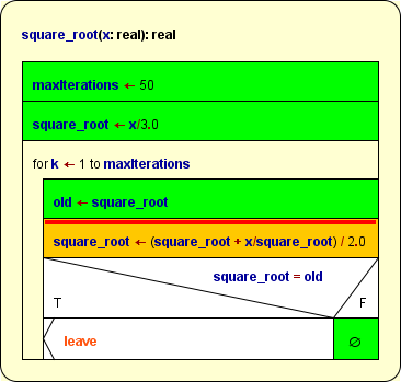
Partially covered function diagram, currently pausing at the breakpoint (execution markup is prioritized over coverage markup).
Coverage Rules
The rules are quite straightforward:
- Simple instructions and Jumps are marked after their first complete execution. Empty elements (e.g. empty FALSE branches of IF statements) also must have been passed before they turn green.
- Structured forking elements (IF statements, CASE selections, and PARALLEL sections) get only marked when all their branches have been covered completely, i.e. turned green.
A specific aspect concerns CASE selections without default branch: Since a missing default branch does not mean that a discriminator value not matching any of the given selector constants were an error – but just lets it pass by –, this structure is actually equivalent to a CASE selection with empty default branch. It is often used if there is no real chance that the discriminator expression might yield a value not among the selectors, but it is not required to be so. Therefore, version 3.25-09 introduced the following distinction: in shallow coverage mode a simplified CASE will be marked as covered as soon as all explicit (i.e. visible) branches are covered, a deep coverage, however, can only be achieved after the hidden default branch had also been passed at least once, such that the following situation may occur (shown in deep coverage highlighting, shallow coverage highlighting would present the entire diagram in green):

- Loop elements turn green on leaving if their respective loop body has been completely covered, i.e. a head-controlled loop will not turn green if the loop body was bypassed.
- For subroutine CALLs there is a deep and a shallow mode. In deep mode, the called subroutine itself is part of the test and must first completely be covered before the CALL element invoking it may turn green as well. The shallow mode, in contrast, assumes that called subroutines will have been tested before and proven to be correct. This does not mean the subroutine wouldn't be tracked, instead it just doesn't require the invoked routine to be covered completely in order to turn the CALL green.
- While the shallow mode treats all subroutines as if they were covered, you may also selectively mark some subroutines parked in the Arranger as formally covered – and adhere to deep mode for the remaining subroutines. (This way, some subroutines are subject to thorough coverage testing while others are not.)
Use the button  "Set Covered" in the Arranger toolbar (or the context menu item "Test-covered on/off" in the Arranger index) to mark a selected diagram as covered. (The button is only enabled in Test Coverage Tracking mode.) A subroutine diagram marked this way will be recognizable by its green outer frame while internal elements are not necessarily highlighted, see image below. (But don't forget that this green colour will only show while one of the visualisation modes "shallow test coverage" or "deep test coverage" is selected!) In the Arranger index, however, the diagrams marked as test-covered will show a green-bordered icon "Set Covered" in the Arranger toolbar (or the context menu item "Test-covered on/off" in the Arranger index) to mark a selected diagram as covered. (The button is only enabled in Test Coverage Tracking mode.) A subroutine diagram marked this way will be recognizable by its green outer frame while internal elements are not necessarily highlighted, see image below. (But don't forget that this green colour will only show while one of the visualisation modes "shallow test coverage" or "deep test coverage" is selected!) In the Arranger index, however, the diagrams marked as test-covered will show a green-bordered icon  while Runtime Analysis is active (no matter, which visualization mode). while Runtime Analysis is active (no matter, which visualization mode).
- The case of recursive CALLs is even a little bit more tricky: If tracked in deep mode, a recursive routine could never become covered since turning it green would require the contained recursive CALL have turned green, which in turn requires the routine be green etc. ad libitum. Hence, a CALL detected to be recursive is ALWAYS tracked in shallow mode to get out of the vicious circle. Note that his does not mean, that the recursive routine itself would automatically be marked, it only gives it the chance!
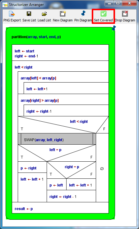
A subroutine diagram in the Arranger window marked via the "Set Covered" button (in red box).
Be aware that the coverage mark around the diagram is only visible while one of the coverage visualisation modes is active. In the Arranger index, however, the respective icon indicates this state with all visualisation modes, provided the Runtime Analysis is enabled.
Remarks
Coverage marks are not stored when saving a diagram to a file. Neither are the count values.
Editing a diagram will clear all collected runtime data and marks, but the numbers are cached in the Undo list. So when you undo the changes then the previous coverage state will be restored and allows you to continue with that constellation.
Complex example
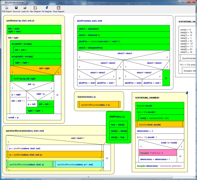
The following three images show phases of a code coverage analysis with Structorizer. The main program is a test frame (diagram at lower right corner in the Arranger window) for a recursive QuickSort algorithm with several nested subroutines (diagrams arranged in the remaining Arranger window area). The first image shows a running test (be aware that there are several "open" subroutine calls at different levels at the same time, recognizable by the orange element colour), the remaining two images show the situation after some more executed tests.
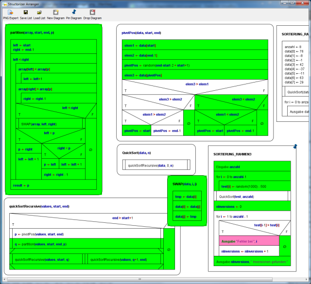

After this last phase in deep mode, all subroutines are completely covered. This does not hold for the test program "SORTIERUNG_RAHMEN3" because the sorting algorithm always worked correctly such that the alert branch (with the pink output instruction) has never been passed. In order to provoke an inversion (i.e. a sorting mistake) detection, routine "QuickSort" might be replaced by a dummy (with same name but not actually sorting) before the next test. This would accomplish the coverage.
Execution Counts (or Transit Counts)
The first one of the two small counts in the upper right corner of the elements represents the number of times the element has been passed during the tests. (All elements with execution counts larger than zero are "test covered", at least in the shallow meaning, see above.) The execution count does not increment before control flow has left the element. This means in case of a structured element (like Alternative, CASE, or loops) that some control path through its substructure must have been completed. Analogously, in mode "Hide mere declarations?" this holds for an instruction being the drawing surrogate for a "collapsed" (hidden) sequence of mere declaratory elements: The excution count will not be incremented before the last of the hidden elements has been passed.
If you select execution counts in the display choice list then the elements will be coloured according to that first count number in a spectral range from deep blue to hot red, where deep blue stands for 0 and hot red for the highest count value over all the involved diagrams.
The following image shows a NEWTON algorithm (used for the computation of square roots), here after the calculation of the square root of 25:

As you can see, the WHILE loop was entered and left only once but the loop body had to be repeated 6 times. So 1 is the smallest and 6 is the highest existing count, and there is nothing inbetween. Hence, only two colours occur. (And since within the range of 0...5 a step of 1 is relatively rough, the blue isn't that dark as one might have expected with value 1.)
This analysis shows e.g. where a code optimisation would be essential if possible (red areas) and where it would not be worth to be considered (blue areas).
Operation Load
The second one of the two small numbers in the upper right corner of an element represents the load of the "atomic" operations (right-hand side of the slash).
If you select done operations lin. or done operations log. then the tingeing of the diagram elements is done by either linear or logarithmic scaling of the number of "atomic" operations, respectively. The logarithmic scale is more sensible if the range of the numbers is very widely spread.
The difference between execution count (number of element transits, see above) and the load of "atomic" operations an element is directly responsible for becomes clearer with the following image, wich only differs from the above situation by the focus of visualisation (where the linear scaling was chosen):

As you may see, here the WHILE loop turned red, too. This is because now every single condition examination counts as an operation (thus costing time). In order to perform the loop body 6 times, the condition has to be examined 7 times (once on first entering the WHILE element, then after each loop execution i.e. before the next iteration, amounting to 7).
Hint: Sometimes users are puzzled by Alternatives showing a high count on the condition but very low operation counts on both branches. This situation will typically occur if one of the branches is empty – an empty element doesn't carry out anything, so it's operation load will always stick to zero! (But look at the transit count in such a case!)
Attribution Rules
The operation loads for the different kinds of elements are:
- Instruction element: Number of instruction lines within the element. Note that
- an empty element will constantly show 0, no matter how frequently ever it may have been passed!
- mere type definitions won't contribute to the operation loads, either, though they are passed at runtime by Structorizer – they are regarded as mere declaratory information usually evaluated by a compiler before excecutions starts. Well, it might of course be disputed why then constant definitions and variable declarations (even without initialization) are counted as operations, because in many compiled languages they are also translated at compile time and won't do anything at run time. But in Structorizer they actually modify the environment state at execution time (computing and assigning a value to the constant or allocating virtual memory to the variable, respectively).
- EXIT element: 1;
- CALL element (on its own): 1 (it costs time to organise the stack descending);
- IF element: 1 for the evaluation of the condition;
- CASE selection: 1 for the evaluation of the distributing expression;
- FOR loop: 1 + n (Initialisation and first test as one operation, increment and test on every repetition);
- WHILE loop: 1 + n (First test and then one further test with every repetition);
- REPEAT loop: n (test after every body execution);
- ENDLESS loop: 0 (no test);
- PARALLEL section: 0 (the synchronisation effort was neglected here);
- TRY block: 0 (the stack unwinding effort is attributed to the throw Jump; if an exception type classification will have to be done in a future version then it might change to 1 in case of catching an exception).
If an element is passed several times then of course the values above will multiply by the number of transits, as you may see with the simple instructions forming the loop body in the diagram above. (The load of the FOR loop should actually be 1 + 2n as it is test plus increment per cycle, which would count separately in an equivalent WHILE loop, but we simplify a little here.)
Note that these loads do not include the loads of the substructure elements. It's only the own contribution of the respective element itself. Only the program (or function) element, i.e. the outer frame, shows the aggregated load of operations performed throughout the entire program / routine. Therefore the parentheses around the load number. The colouring of the program / the routine, however, does not reflect the aggregated load but is based on the net operation load which is used to be zero (deep blue in the above image).
From this colouring you may learn where most of the time is consumed.
Note: With recursive algorithms, the operation loads give only a notion of the time distribution on the top level (or the current level, on interruption). Otherwise the overall sum wouldn't be correct since the operation load of the analogous elements at called levels will already have been aggregated in the recursive calls being visible in the same context. This way, it is possible that the execution count of an instruction in a recursive routine is greater than its shown operation load, because the execution count represents all copies of the element whereas the operation load is bound to the currently visible level.
If you collapse a structured element, then its displayed load of operations will increase by the operation loads of the contained elements – as if they were melted together. The tinge of the element will not change, however.
So for the WHILE loop in the example above this would mean a load of 7 + 6 + 6 + 6 = 25. In this case (as the loop elements are flat instructions), it would be the number also presented by the following aggregated mode.
For sequences of declarative elements in display mode "Hide mere declarartions?" is similar like for collapsed structured elements, but that the background colour does differ from the normal display mode (where each element of the sequenec stands for itself) – the drawing surrogate for the declaration sequence will appear as its amalgamation (and be tinged like in the Total Operations Load visualisation mode).
Total Operations Load
If you select one of the visualisation modes total operations lin. or total operations log. then the tingeing of the diagram elements is done by either linear or logarithmic scaling of the aggregated load of operations, respectively, i.e. the load of structured elements also recursively includes the loads of their respective substructure. The logarithmic scale is more sensible if the range of the numbers is very widely spread.
The aggregated operation numbers on structured elements will be enclosed in parentheses to remind that these are composed data.

On collapsing elements, the load won't change of course (it just loses its parenthesis), nor will the colour.
This mode is fine to visualise the hierarchical aggregation and load distribution – it is all calculated already. The program element tells you the overall number of (fictitious) unit operations to accomplish the computation and may serve as an estimate for time complexity if you find the functional relation to the number or size of data to be processed.
Complex Example
Again, the colouring shall also be demonstrated with the complex example of a recursive quicksort algorithm with several nested routine levels.

Recursive QuickSort algorithm composed of several subroutines, in Execution Count mode

Recursive QuickSort algorithm composed of several subroutines, in local Done Operations mode
Freedom of Choice
Once the Runtime Analysis has begun you may freely switch among the different visualisation modes, export the coloured diagrams to different graphics formats, print them, arrange them, etc. until you unselect the checkbox "Collect Runtime Data", in which case all collected data are cleared and the display returns to standard mode.
As already stated for the test coverage mode, however, saving a diagram in its native file format will not store any of the gathered results. So if you want to document the results, you must export the diagram(s) as a picture. |